|
Integrating Wildland-Urban Interface (WUI) Fire Models with
Geographic Information Systems (GIS)
Camp Swift, Texas Prescribed Burn Geospatial Data Integration
(National Institute of Standards and Technology (NIST) Fire Research Grant 60NANB11D173)
Last Updated July, 2015.
Acknowledgments: The work described below was in part performed under a NIST Fire Research Grant. The data presented below are all derivative products of data collected by NIST and the United States Forest Service (USFS) in cooperation with numerous organizations. In particular, the efforts of Alexander Maranghides and William Mell are acknowledged particularly in regards to making the data available for the effort presented here.
Data Disclaimer: Geospatial Measurement Solutions, LLC (GMS) makes no representation of any kind, including, but not limited to, warranties of merchantability or fitness for a particular purpose or use, nor are any such warranties to be implied with respect to the information, data, or software furnished herein. In no event shall GMS, its employees, or partners become liable to users of the data presented herein, or to any other party, for any loss or damage, consequential or otherwise, including but no limited to time, money or goodwill, arising from the use, operation or modification of the data or information presented herein. In using the data or information provided by GMS, users assume the risk for relying on such data or information, and further agree to indemnify, defend, and hold harmless GMS, it employees, and partners for any and all liability of any nature arising out of or resulting from the lack of accuracy or correctness of the information or data, or the use of the information or data presented herein. Finally, in using the information and data presented herein the user acknowledges that the user is responsible for assessing the accuracy and reliability of the data or information provided. By downloading any data, using any information, or exercising any software on this website the user accepts the above restrictions and information usage.
|
Zoom in on above map to view pre-fire, during-fire, post-fire imagery by clicking on "+" button at upper right.
If zoomed out too far and place is lost, refresh web page and zoom in again.
VIEW ABOVE MAP IN FULL WINDOW
|
Background
On January, 15, 2014 a series of prescribed burns took place at Camp Swift, Bastrop County, Texas. A primary goal of the prescribed burns, conducted jointly by over 14 organizations, was to build and asses various technologies for characterizing pre-fire, during-fire and post-fire conditions to provide a better understanding of fire behavior and the conditions under which relevant fire behaviors occur. This information is required to help build the Exposure Scale developed by Maranghides and Mell (2012), which could provide a method to rate a WUI community's susceptibility to wildfire. Additionally, the data provides inputs required for fire behavior models such as the Wildland/WUI Fire Dynamics Simulator; thereby providing data sets for fire model validation. Numerous data were collected both spatial and tabular requiring processing, integration and assessment to facilitate further analysis. Additionally, data needs to be integrated into fire model input files to facilitate model simulations for the assessment of fire model performance.
A short film of the burns is available, which documents certain aspects of the prescribed fire. Geospatial Measurement Solutions (GMS) was called in after these burns to organize, process and integrate certain spatial data while assessing improvements to geospatial science and technology applications and data management for future burns. Listed below are the spatial data derived by GMS to date under the NIST Fire Research Grant from the NIST/United States Forest Service (USFS) acquired raw data. These data are also being used to develop tutorials for software that integrates GIS data with fire models.
|
Digital Surface Models & Topography
Light Detection and Ranging (LIDAR) data was acquired for the study area from the Texas Natural Resources Information System (TNRIS) program. Limited information was included with the raw LAS files, which were provided classified for ground points and flown in 2008. The point spacing was estimated at approximately 1 to 1.5 meters. A bare earth digital elevation model (DEM) was created from the LAS data by converting a Triangulated Irregular Network (TIN) of ground points to a geotiff. Additionally, a canopy height model (CHM) was also created by classifying unclassified points to building and vegetation classifications and performing the same transformation as with the DEM. The CHM, however, due to the data being acquired in 2008 might not reflect vegetation and building conditions currently present on the site as is evident in some locations. The CHM is likely not required as the vegetation mapped in the CHM data set is shrub and tree species not present in the plots nor was their evidence these far afield vegetation species had consequences for wind in plot 1. The CHM data set is provided for GIS/Model integration demonstration purposes.
The bare earth DEM and the CHM can be download below:
It should also be noted that due to the active management of the field it is possible the topography represented in the 2008 LIDAR data does not represent the current topography in some locations.
Figure 2 shows contours derived from the bare earth DEM overlaid on a hillshade of the DEM for the study site. The plots were relatively flat but did slope gently from east to west. Plot 3 contained a knoll on the northwest part and plot 1 also contained a knoll on the southeast part of the plot. There was also a knoll to the west of plots 1 and plot 2.
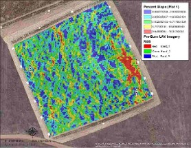
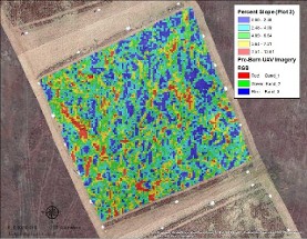
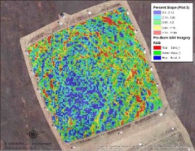
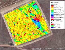
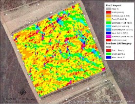
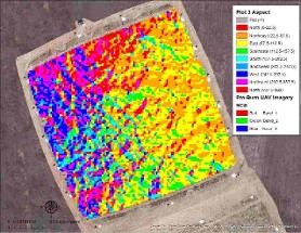
Figure 3 shows percent slope for plot 1. Slopes ranged from 0 percent to over 18% on the west side of the knoll and small select other locations. Figure 4 shows percent slope for plot 2. Slopes ranged from 0 percent to over 13 percent. Figure 5 shows percent slope for plot 3. Slopes ranged from 0 percent to over 11%. Figure 6 shows aspect for plot 1. Figure 7 shows aspect for plot 2. Figure 8 shows aspect for plot 3. Aspect and slope were derived using ArcGIS™ SLOPE and ASPECT functions in the Spatial Analyst™ extension.
|
Study Area
Camp Swift is a Texas Army National Guard training site located in Bastrop County, Texas. Bastrop County was the site of the worst Wildland-Urban Interface (WUI) disaster in Texas History. The Bastrop County Fire Complex destroyed over 1,500 homes in September of 2011. NIST and the USFS partnered with the Texas A&M Forest Service to perform a post-fire assessment of the Bastrop County Complex Fire. More information on the Bastrop Fire can be found in various articles and press releases. This collaboration lead to the research burns at Camp Swift. Research prescribed burns such as the Camp Swift burns have potential to provide valuable information to first responders regarding fire behavior; thereby possibly allowing for the development of more efficient and effective WUI and wild land mitigation advice. Integrating the data in a GIS environment allows for exploratory data analysis as well as a means to examine the feasibility of creating fire model inputs from spatial data and linking fire model outputs back to a GIS for further spatial analysis.
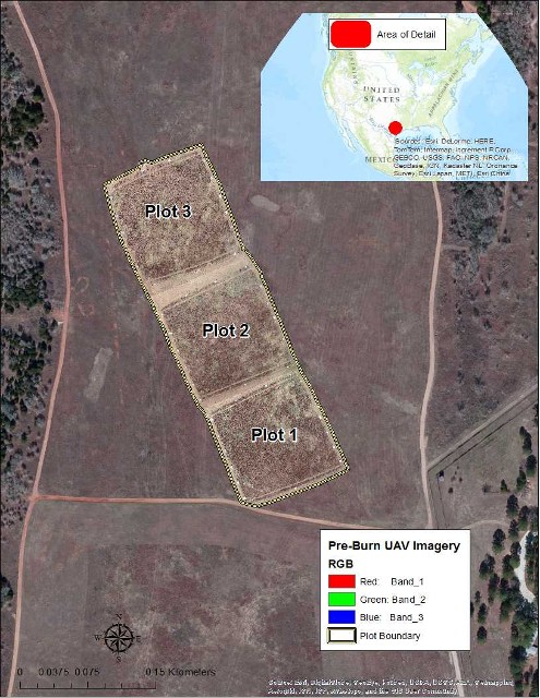
The location of the research prescribed burns are shown in Figure 1. An open field consisting of various grass and fob species was divided into three plots of roughly equal size. This field is heavily managed with fuels changing dramatically from year to year. Consequently, acquisition of timely imagery was a necessity to correctly map the fuels on the study site. Fuels were mowed around the edge of each of these plots as shown in Figure 1. Plot 1 is a roughly 1.2 hectare plot with sides of length equal to approximately (plot sides are not exactly straight lines with length being measured from plot corner to plot corner on georectified imagery described below) 109 meters on the east side, 105 meters on the north side, 100 meters on the west side and 111 meters on the south side. Plot 2 is a roughly 1.2 hectare plot with sides of approximate length of 109 meters on the east side, 110 meters on the north side, 103 meters on the west side and 108 meters on the south side. Plot 3 is a roughly 1.2 hectare plot with sides of length 111 meters on the east side, 108 meters on the north side, 105 meters on the west side and 106 meters on the south side. Lengths were measured from georectified imagery and not orthorectified imagery and consequently do not represent true distances.
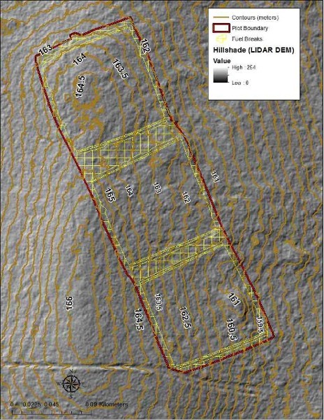
Figure 2: LIDAR derived topographic contours overlaid on hillshade of LIDAR bare earth DEM with plot boundaries and fuel breaks. Elevations varied from approximately 159.5 meters to 164.5 meters in plot 1. In plot 2 elevations varied from approximately 161 meters to 165.5 meters. Plot 3 elevations varied from approximately 162 meters to 164.5 meters.
|
|
Instrument Locations and Fuel Sampling Sites
|
Numerous instruments were placed in and around the prescribed burn plots. Figure 9 shows the spatial location and number placed of various instrument types. Locations of instruments, fuel sample sites and ground control points where recorded with a Trimble GeoXH 6000 GPS receiver and differentially corrected using one base station and Pathfinder Office Software.
Fuel sampling occurred outside of the plots prior to the burns with some sampling occurring inside the plots after the burn. Pre-fire sampling inside of the plots did not occur due to concerns this destructive activity could have consequences for fire behavior. Additionally, foot travel inside the plots was limited to only essential placement of devices in order to reduce any potential altering of fuels, which might have consequences for fire behavior.
There were 7 pre-fire fuel sampling sites, the general location of which are shown in Figure 10. Exact locations of destructive sampling sites were not provided for pre-fire sampling locations, though many of these are visible in the imagery. There were 47 post-fire sampling locations included in the plots. The location of these sampling sites is also shown in Figure 10. Vegetation unconsumed by the fire was recorded in these sampling locations and might be used as a coarse means of assessing the accuracy of fuel classifications in plot 1 as described in the Fuel Classification section below. Fuel ignition line locations were also recorded using the GPS.
The placement of ground control points focused on placement of easily recognized objects (i.e., well known points) for video imagery. Two sets of ground control were placed around each plot. Sixteen fire shelters where placed around each plot to use as ground control for visible video stills. Additionally, sixteen metal trays filled with burning charcoal were placed around each plot for thermal imagery ground control points.
Shapefiles with associated metadata (some still being developed) representing the above data sets can be downloaded using the links below:
|
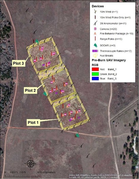
Figure 9. Location of measurement devices for prescribed burns showing UAV acquired imagery overlaid on Environmental Systems Research Institute (ESRI) World Imagery Map Service.
|
|
KMLs representing the above data sets can be downloaded using the links below:
An interactive map showing the placement, ID and type of various prescribed fire devices and features can be viewed here.
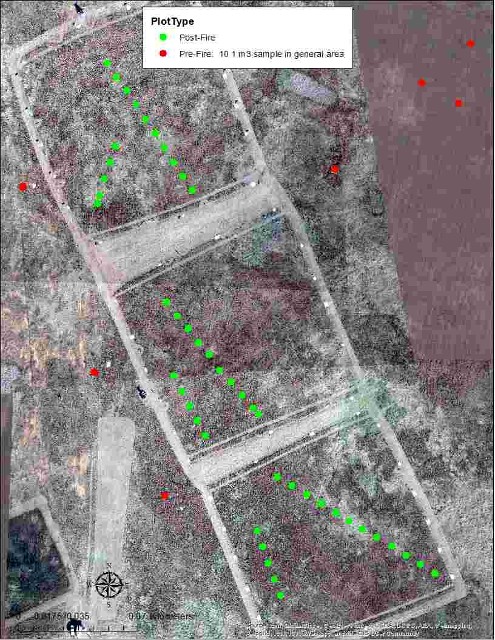
Figure 10. Location of fuel sampling locations for pre-fire and post-fire samples.
|
Unmanned Aerial Vehicle Imagery
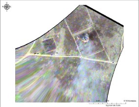
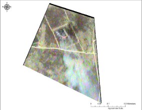
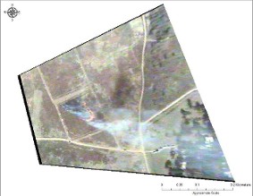
Still and video imagery for the study site was acquired for pre-fire, during-fire and post-fire conditions. A Cannon EOS Rebel T3i was used to acquire pre-fire imagery. A Canon EOSM was used to acquire post-fire imagery. Pre--fire and post-fire still imagery was acquired at what appeared to be close to NADIR angles. Various video sensors where used to capture during fire behavior including visible and thermal video cameras. Information to perform complete orthorectification or use full motion video was not provided. Consequently, ground control data was used to georectify the imagery and video frames using ArcGIS™.
Various georectified Geotiff image data sets can be downloaded using the links below:
Google earth KMZ files of some georectified Geotiff images can be downloaded using the links below:
Various videos of georectified video stills can be downloaded below.
Videos are provided for initial assessment. Some apparent shifts in fire direction displayed in the video are a result of different viewing angles and large gaps between frames. The above videos should be used with caution. Georectification of additional video frames is likely to be required for full assessment of the fire. Additionally, video frames should be assessed in conjunction with other data such as spatial representations of wind fields as demonstrated below. Nonetheless, the above videos provide information for exploratory data analysis to guide future efforts and evaluate the geospatial science and technology utilized in the burns.
|
|
It is the rectification of the imagery that allows for the data to be integrated and analyzed concurrently (i.e., GIS overlays). The above videos provide rudimentary examples of data integration that could be used for qualitative analysis. Nonetheless, data rectification, transformation and organization into formats suitable for viewing in a spatially aware environment such as a GIS is a necessary step before incorporation into Computational Fluid Dynamics (CFD) models such as WFDS-Physics Based (WFDS-PB) or empirical models such as WFDS-Level Set (WFDS-LS) can occur.
Nonetheless, care should be taken in analysis of during fire georectified imagery particularly regarding tall features such as smoke plumes or high flames. Figures 11 through 13 show three video frames and describe the direction these video frames were taken from during the prescribed fire in plot 1. It can be observed in these figures how the smoke plume appears to move from southwest to southeast, indicating a possible change in fire direction. It is possible that there were topographic, fuel or weather conditions that caused a somewhat west to east shift in fire direction. However, this cannot be assessed accurately using the smoke plumes in these images, which has large distortion for tall features.
The magnitude of the distortion in oblique imagery will increase with greater oblique angles of the imagery. This can clearly be seen in the curved nature of the smoke plumes. Figures 11 through 13 all show a curvature to the smoke plume that increase with height away from the direction of the image acquisition. This distortion, can also be seen in the fire line, though far less dramatic in most cases, leading to the appearance of the fire line moving somewhat in the direction of the image acquisition with some distortions in the measured location of the fire line depending on the angle of the camera at the time of acquisition and the height of the flames. Consequently, ancillary data such as ground measurements should be used to confirm small scale changes in fire direction. Larger scale changes, such as occurred in plot 3, are more apparent in the oblique imagery. However, larger scale changes that produce higher flame heights could also have significant distortions present.
Fuel Classification
One single UAV acquired georectified pre-fire image for plot 1 was used for image classification. Initial classifications were conducted on this data set to demonstrate potential work-flows, which might produce useful inputs for WFDS simulations. Additionally, these classifications might be compared visually to fire behavior observations to determine if fuels had consequences for fire behavior. Finally, these classifications will allow for visual comparison to field sampled data to help determine requirements for improving remote sensing and field sampling integration to provide improved data for characterizing fire behavior and performing fire model validation.
Unmanned Aerial Systems (UAS) such as the NIST/USFS system might be calibrated, configured and synchronized to produce orthorectified image mosaics, point clouds of image features and other products useful for fuel classifications. Commercial software products are available to produce these image derivatives with most of the effort being in collection of ground control, and synchronization and calibration of equipment. Appropriate flight parameters are also required. The exact contribution of each component is mission dependent.
It is also possible to estimate interior camera geometry parameters when lacking a camera calibration report to produce an orthorectified image product. However, many commercially available UAV image processing software packages provide utilities for camera calibration. Nonetheless, establishment of ground control outside (and inside) the plot boundaries will help in future orthorectification and accuracy assessment efforts related to acquiring imagery with a UAS. Nonetheless, given the relatively low camera angle, relatively flat topography and need for imagery only within the plot boundary; the acquired imagery was only georectified. If orthorectified imagery is required and necessary information is available to perform this orthorectification, the same automated work flows presented here can be conducted for fuel classification. Furthermore, the ground control and image coordinate relationships have been established for some of the images reducing much of the effort involved.
Regardless, of the photogrammetric mapping methods employed, essential to any remote sensing effort is ground control. The required ground control was collected by the USFS Fire and Environmental Research Applications Team (Vihnanek et al., 2014). This effort utilized the species classifications in the various plots. A great deal of additional information was collected by the USFS team regarding material properties of vegetation. Further analysis of field sampling of material properties of vegetation will be essential to the fire behavior characterization and model validation effort.
|
|
Due to logistical difficulties associated with prescribed burns the field sampling had to occur prior to image acquisition for some identified vegetation species. This makes it difficult to correlate field estimates of material properties of vegetation (e.g. biomass) with remote sensing data. Additionally, correlation of imagery acquired when vegetation is in senescence, as was the case with most vegetation at these study sites, with biomass estimates is difficult and would be size and species dependent if possible at all. The field data, however, did allow identification of some of the prominent vegetation species in the study area. The prominent species identified through pre-fire field sampling consisted of Little Bluestem (Schizachyrium scoparium), and an unknown to GMS species of the genus Aristida (Threeawn). Other miscellaneous grasses and forbes where identified in pre-fire sampling outside of the plot. Post-fire sampling in the interior of the plots did identify some type of plant identified as Broomweed as well as forbes.
Little Blue Stem was visually identifiable in the pre-fire imagery for plot 1 as reddish vegetation. Additionally, Threeawn could clearly be identified as gold with some patches of yellow to green colored vegetation thought to also contain Threeawn. It is believed the remainder of the area was either open areas with forb understory, and/or Broomweed. The potential spectral differentiation between at least some vegetation allowed for the use of object oriented image classification procedures. Figure 14 shows the work flow employed for extracting vegetation by species for plot 1.
Fuel breaks and plot boundaries were first manually digitized. Automated extraction of fuel breaks was not successful. Fuel breaks appeared to retain distinctive textural and spectral characteristics of the mowed vegetation, some of which was extracted in initial classifications, which made it difficult to extract as a complete entity. This was also evident in the post-fire imagery where locations in the fuel breaks that had a reddish hue (i.e., contained Little Blue stem prior to the mowing) seemed to have more burning from escaped fire in the plots compared to other fuel break locations.
|
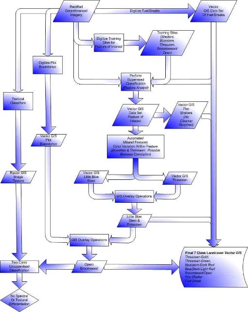
Figure 14. Workflows for development of 7 class landcover vector GIS data set.
|
|
For each feature of interest a small number of training sites were digitized from the imagery. Fire shelters, Threeawn and Little Blue Stem where readily identifiable in the imagery. Supervised classifications where used with these training sites in Feature Analyst™ to extract the feature of interest. Fuel shelters where extracted successfully with no cleanup required. Training sites for Little Blue Stem and Threeawn focused on dark red vegetation and gold vegetation, respectively, initially. Automated missed feature functionally was then employed to delineate lighter red areas of Little Blue Stem and green to yellow areas as what was initially believed to be Threeawn. Various GIS overlay operations were then utilized to produce the Threeawn and Little Blue Stem vector GIS data set. More GIS operations were utilized in conjunction with the plot boundary GIS data set to identify the remainder of the areas in the plot. These areas where estimated to be either open areas with a forb understory or areas of Broomweed. Textural classifiers (textural classifiers were examined for other species delineations with no visual improvement in extractions) were employed to asses if an unsupervised classification could discern spectral or textural differentiation within the "Open/Broomweed" classification. The unsupervised classification did not identify any significant differentiation, which does not imply there is not a differentiation in material properties of vegetation relevant to fire behavior only that there were no spectral or textural characteristics that allowed for differentiation. Consequently, the fire shelter, fuel break and two class Threeawn, two class Little Blue Stem and Open/Broomweed landcover classes where combined to form the landcover data set for plot 1 shown in Figure 15.
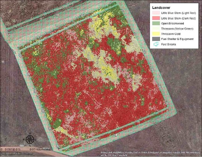
Figure 15. Plot 1 seven class landcover vector data set.
Lacking pre-fire plot data and the exact locations of pre-fire fuel sample locations, qualitative efforts were employed to possibly relate field sampled material properties of vegetation to remote sensing classifications. The two classes derived for Little Bluestem were based on visual observations of lighter red Bluestem producing shadows that appear to be shorter compared to dark red Bluestem. If a relationship between vegetation height and biomass could be established with field data it might represent a means to correlate field sampled biomass estimates for Bluestem with feature classifications. The Bluestem color classes could also be subdivided further if field data indicates such a relationship. Threeawn, also showed spectral variation within different areas but it was less clear if this represented a difference in structural stage, a difference in vegetation density or if the Threeawn (Yellow/Green) fuel class represented some other species or mix of species.
A shapefile and google earth KMZ file of the vegetative fuels data set can be downloaded at the links below:
Post-fire fuel sampling can also help to provide some assessment of the accuracy of the fuel classifications derived for plot 1. Post-fire fuel sampling examined vegetation species remaining after the burn. It is assumed that lack of a species present does not indicate that the species was not present during the pre-fire environment. However, the presence of a particular species in the post-fire environment can help to identify errors of omission in the above described vegetation classifications.
Table 1 portrays the error matrix comparing post-fire field sampled vegetation in plot 1 with remote sensing classified vegetation. It is important to note that the post-fire field sampling could only assess vegetation that was not completely consumed by the fire leading to many possible biases in the assessment. For example, there were no post-fire fuel samples that identified Threeawn, which might indicated this fuel was mostly consumed by the fire in the sampling locations. Additionally, assessment of the remote sensing classified imagery would be better accomplished with samples that were evenly distributed between classifications, an impossibility at this burn given logistical constraints. Finally, there is only a limited number of samples in plot 1 but assessment of all future classifications in all plots would provide a greater sample size.
Despite the shortcomings of the accuracy assessment presented here it does provide some useful information. For example, it can be seen that Little Blue Stem classifications had a 100% user accuracy and 75% producer accuracy. It should be noted that all three of the points of field sampled Little Bluestem classified as "Open/Broomweed" or Threeawn were less than a half meter away from larger patches of classified Bluestem. This is well within the combined accuracies of the above data indicating the possibility of the producer accuracy for Little Bluestem being caused by spatial misalignment between the field samples and the remote sensing classified imagery. The same possible spatial misalignment coupled with threeawn possibly being completely consumed could also explain the low user accuracy and producer accurcy (could not be calculated) for Threeawn. Also, three of the threeawn locations misclassified as open/broomweed where of the yellow/green classification.
|
Table 1: Error matrix describing errors of omission, errors of commission, mapping accuracy per fuel classification and overall fuel classification,
|
Post-Fire
UAV Imagery Derived Fuel Class
|
Field Sampled Fuel Class |
| Little Bluestem |
Threeawn |
Open/ Broomweed |
Total |
User Accuracy
|
Producer
Accuracy
|
| Little Bluestem |
9 |
0 |
0 |
9 |
100 |
75 |
| Threeawn |
1 |
0 |
3 (Threeawn:yellow/green) |
4 |
0 |
NA |
| Open/Broomweed |
2 |
0 |
2 |
4 |
50 |
40 |
| Total |
12 |
0 |
5 |
17 |
Overall Fuel Classification = 65% |
|
Consequetly, the "Threeawn (yellow/green)" fuel classification contains the most ambiguity and coupled with the "Open/Broomweed" fuel classification will likely be the most difficult for which to ascertain material properties of the vegetation type given the field data. The overall fuel classification is calculated at 65%. This number, however, should be viewed with caution given the limited sample size and the information provided above. Table 2 shows the percent area in plot 1 occupied by each fuel classification type. These percent areas include the buffers at the north and south side of each plot. Table 2 might be used to understand which areas of plot 1 might not have representative field samples.
|
Table 2: Percent area of each fuel classification found in plot 1 with buffers.
Fuel Classification
|
Percent Area
|
| Bluestem (Dark Red) |
54.0% |
| Bluestem (Light Red) |
11.0% |
| Open/Broomweed |
21.7% |
| Threeawn (gold) |
3.7% |
| Threeawn (yellow/green) |
9.6% |
|
Wind
Wind is a driving factor in most fires. As can be seen in Figure 9, many instruments were placed around the burns to record wind conditions. Most GIS packages provide tools for animation that can serve as a valuable method for analysis of wind in conjunction with other data sets. An example animation for wind (3m anemometers), with some IR video stills, vegetation and topography can be downloaded below:
- Wind, vegetation and fire animation.
Incorporation of other wind sensors with additional georectified video still images would provide more information. Initial visual examination of data such as provided in the video above can help to guide more in depth analysis of the prescribed burn. Incorporation of 10m anemometers and SODAR wind data in the above animation might also help.
The wind data animated above was collected by the Rocky Mountain Research Station's Fire Sciences Laboratory in Missoula, MT (Butler et. al. 2014).
GIS, Fire Behavior Characterization and Fire Model Integration
The complete evaluation of fire behavior at the Camp Swift research burns requires integration of all spatial and tabular data some of which was not utilized in the effort presented here. This type of integration is a necessary step in assessment of any prescribed burn, particularly in regards to characterizing fire behavior and exposure conditions to help build the Exposure Scale developed by Maranghides and Mell (2012). Spatial data sets representing wind measurements along with more georeferenced video still frames than assessed to date might help better quantify fire behavior in regards to weather, topography and fuels. Additionally, ground videos were located in various locations throughout plot 1 along with fire behavior instrumentation and thermocouples, all of which can provide additional information regarding fire behavior characterization that are not assessed here. Nonetheless, the data presented here provides a foundation for future more in depth efforts.
Furthermore, the above data does allow for initial exploratory data analysis regarding fire behavior, which might help guide future data processing and analysis efforts. Ultimately, the processing and analysis require an understanding of the scale of fire behavior of interest to ensure pertinent aspects of the prescribed burns are being assessed both in regards to fire model validation and development of the Exposure Scale. GIS type environments are well suited for integrating and assessing data of different scales but care must be taken to ensure results are described at scales appropriate to the given data. The scale of interest for the phenomena being studied should also be known and described to Geospatial experts performing data integration for particular cases.
Finally, GIS provides a means to integrate data allowing for evaluation of the use of geospatial data in various fire models including WFDS-LS and WFDS-PB models, empirical and physics based models, respectively. Fire models outputs can also be viewed and analyzed in a GIS environment to facilitate integration and assessment with other data sources. This section presents exploratory data analysis conducted to date related to fire behavior as well as initial efforts related to GIS and Fire Model integration.
Plot 1 Fire Behavior Characterization (Exploratory Analysis)
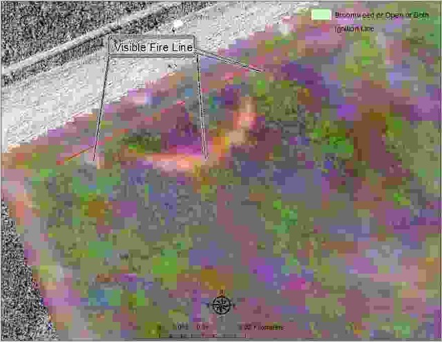
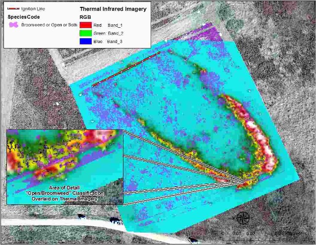
Complete fire behavior characterization requires integration of all data collected for the Camp Swift Research Burns. Some observations, however, can be made using the above partial data in regards to fuel, topography and fire behavior. For example, Figure 16 shows the "Broomweed/Open" vegetation classification overlaid on one video frame from the visible during fire video. As can be seen in Figure 16, larger, contiguous areas mapped as "Broomweed/Open" did have less visible flame areas compared to areas with other fuel type classifications. This did appear to have consequences for fire behavior early in the ignition where splits in the fire line are seen coincident with these locations. It is, however, unknown if this is due to some change in material properties of the vegetation or if these areas are basically lacking in fuels. This might be ascertained from discussions with on the ground observers. These areas of "Broomweed/Open" appeared to have resulted in the ignition line not being set in these locations. When the ignition line was set the head fire did appear to be able to travel through some areas classified as "Broomweed/Open" but these where smaller in size. Additionally, fire behavior under a few meters horizontal resolution might not be captured in visible or thermal video stills.
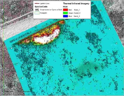
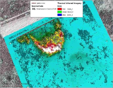
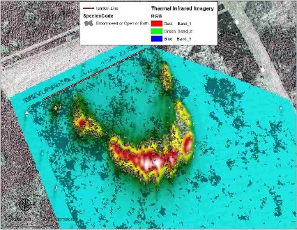
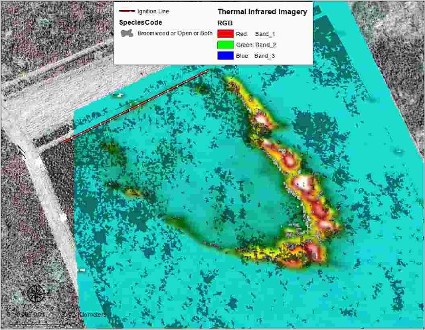
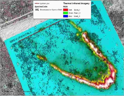
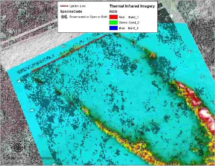
This same trend of "Open/Broomweed" classified areas reducing fire intensity can be seen in various thermal infrared video georectified still frames taken after the frame shown in Figure 16 and shown in Figures 17 through 22. Light blue in Figures 17 through 22 generally shows area of no heat release or much less, comparatively, from the fire. Dark blue are areas mapped as "Broomweed/Open" with 50% transparency to see the fire line below the fuel classification. As can be seen in Figures 17 through 22, large continuous patches of vegetation mapped as "Broomweed/Open" did show less areas of lower to no intensity fire. This might be most clearly portrayed in Figures 21 and Figures 22. Figure 21 shows a relatively continuous flanking fire line on the east side of the fire and Figure 22 shows this continuous fire line being broken at areas coincident with the mapping of vegetation classified as "Broomweed/Open". This provides some evidence that this vegetation (or lack of vegetation) classification might have had material properties that resulted in lower intensity fires.
Comparison of Figure 19 and Figure 20 also shows a change in fire behavior on the west flanking fire where Figure 19 shows a higher intensity flanking fire compared to Figure 20. There is no classified vegetation change associated with this difference in observed fire intensity as the vegetation is burning through areas classified as Little Bluestem and the areas classified as "Broomweed/Open" all coincide with distinct breaks in the fire line. It is possible that some other factor caused this change in fire behavior, such as wind.
It should also be noted that the two frames in Figure 19 and Figure 20 were taken at opposite camera angles. The camera was located to the east of the plot in Figure 19 and the west of the plot in Figure 20. It also seems that the the image frame shown in Figure 19 might have been taken during a period of relatively high flame heights, which exaggerated the heat release being portrayed to the west in this image. In fact, the western edge of the heat displayed in Figure 20 is 8 meters further to the west than the western edge of heat portrayed in Figure 19, which portrays a video frame taken earlier in the fire than the video frame shown in Figure 20. This points out that certain aspects of the fire might be sensed at different resolutions and accuracies from oblique imagery depending on the geometry of the image acquisition.
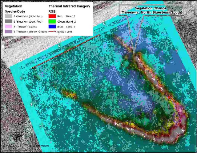
A possible change in fire behavior with mapped fuel vegetation classifications can also be seen in Figure 23. This figure shows the same thermal video frame shown in Figure 21 but with Threeawn and Bluestem mapped vegetation polygons overlaid on the imagery. As can be seen in Figure 23 there is a clear and abrupt difference in the size of the east flanking fire line in areas mapped as Bluestem compared to areas mapped as Threeawn with the Threeawn areas showing less areas of heat. However, other factors might contribute to the difference in intensity including distance from the head fire.
Other possible examples of change in fire behavior coinciding with changes in fuels exist in other thermal and visible video frames that have not been georectified to date. These include flanking fires transforming to head fires, fire crossing fuel breaks at vegetation specific locations and other examples. Some of these examples might also help describe the relative spatial accuracy between data sets. For example, Figure 24 shows a single thermal video frame with the "Open/Broomweed" fuel classification overlaid on top. This georectified video still shows the fire coming to the end of the plot and the spatial coincidence of the "Open/Broomweed" fuel classification at the end of the plot. This indicates that the relative accuracy between pre-fire and during-fire imagery is fairly good but additional oblique frames that have not been georectified to date might help to provide additional information regarding relative spatial accuracy between data sets.
As mentioned above, Plot 1 had little topographic relief. The single knoll found in plot 1 is the largest topographic feature found in plot 1. Figure 25 portrays another method of portraying topography. Figure 25 shows topographic flow direction derived in ArcGIS™. For each grid cell in the input terrain the flow direction is calculated and displayed. Many small scale topographic features are portrayed in red in Figure 25 where red shows flow directions to the Southwest, West and Northwest (i.e., the opposite direction of the predominant topographic flow in the plot). As can be seen in Figure 25 most of the reddish areas are small in area and beyond the scale of what can be discerned from the aerial videos. However, the knoll in plot 1 can be clearly seen as a larger feature, which might cause changes in fire or local weather behavior. The images georectified to date do not focus on the fire around this knoll but georectification of further images along with examination of ground images (a go pro camera was placed on top of this knoll) might help identify if this feature caused changes in weather or fire behavior.
|
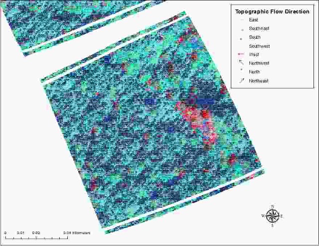
Figure 25: Topographic flow derived in ArcGIS for plot 1.
|
GIS/Fire Model Integration
GIS is a powerful tool for integration and assessment of prescribed fire data but direct analysis of physics based aspects of fire behavior are beyond the capabilities of GIS platforms. Consequently, physics based fire models such as WFDS-PB, which are capable of simulating complex fire behavior, are logical tools for use in assessment and integration of prescribed burn data. These fire models, however, are in the early stages of development with validation ongoing. Collecting and deriving data for inputs to models such as WFDS at prescribed burns might be invaluable for certain aspects of the validation and evaluation efforts of WFDS-PB, WFDS-LS and other fire models.
As science and technology progresses the synergistic use of prescribed burn data (weather, fuels, topography and other required data), GIS and fire models might provide feedback mechanisms to improve processes and worflows throughout the life cycle of the prescribed burn effort, from planning to final analysis. This can lead to improved fire models that might provide a better understanding of environmental characteristics pertinent to measure in a prescribed fire environment and information on how best to integrate spatial and tabular data to portray this understanding. This type of information could aid in development of appropriate test methods for building materials and in gaining a better understanding of fire prone landscaping characteristics (Maranghides and Mell, 2012) while allowing for development of spatial based tools to apply this information and knowledge in real world environments. Standard test methods appropriate to representative wildland environments coupled with science based spatial tools have potential for improving and implementing building and landscaping codes and standards; thereby better protecting lives and property in the WUI and wildlands.
In this study, the above data was integrated using a prototype software application developed under the GMS awarded NIST Fire Research Grant. This represents the first time that geospatial data (presented above) for a prescribed burn including topography is being examined for integration with WFDS-PB and WFDS-LS fire models. This is the only current data set available, to the author's knowledge, to perform such an activity. Consequently, this is the only data set available to WFDS modelers to provide improvements to the one single model validation data set currently available (Australian grassland fire experiments of Cheney et al.1993). Several demonstrations and model input files are presented below to aid WFDS modelers in initial examination of the data to guide future efforts. These demonstrations are also provided to inform modelers of potential issues with transforming GIS data to WFDS inputs.
The basic operation of transforming GIS data to WFDS inputs involves transforming 2-Dimensional (2-D) or 2.5-Dimensional (2.5-D) data structures to 3-Dimensional (3-D) data structures. In many ways this is a simple transformation. However, complexity can increase rapidly as the amount and variation of data being transformed increases. In the case of the Camp Swift data it does represent a relatively simple transformation, initially at least in terms of terrain.
Nonetheless, the transformation, depending on desired model grid cell resolutions, can have consequences that could be examined. Additionally, traditional methods for scaling 2 and 2.5D data to higher resolutions might not be appropriate for physics based fire models. Finally, transforming 2.5D data to a Cartesian block data structure such as used in Fire Dynamics Simulator (FDS) will inevitably produce stair stepping artifacts (McDermott et al., 2010). New data structures (i.e., not cartesian block geometries) for WFDS might be required to allow for a smoother transformation between 2.5D data and 3D data. FDS developers are examining the use of triangle facets (FDS Road Map, 2014) to account for complex geometries present in many wildland and WUI environments.
Figure 26 shows two representations of the topography in plot 1 displayed in Smokeview. Figure 26a shows the 2.5-D terrain (i.e., a 2-D raster data set with each pixel containing an elevation value) transformed to a Cartesian block resolution of 1mX1mX1m (X,Y,Z). Figure 26b shows the 2-5 D terrain transformed to a WFDS Cartesian block resolution of 1mX1mX0.1m. As can be seen in Figure 26a, transforming the LIDAR data to 1m resolution in the vertical (Z) direction results in the creation of stair stepping that is not as evident at finer vertical resolutions shown in Figure 26b. This transformation essentially produces artificial topographic features that might lead to artificial changes in the wind field (FDS Road Map, 2014) or have other consequences for simulated fire behavior.
|
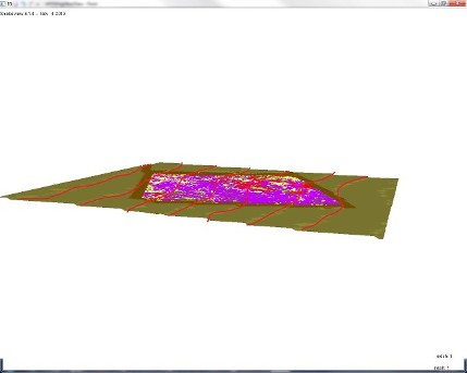
Figure 26a. WFDS inputs at 1mX1mX1m (X,Y,Z) grid cell resolution viewed in Smokeview. Red lines highlight stair stepping (i.e., flat plateaus with abrupt rises in elevation produced when using a vertical resolution of 1 meter).
|
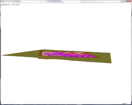
Figure 26b WFDS inputs at 1mX1mX0.1m (X,Y,Z) grid cell resolution viewed in Smokeview. Stair stepping seen at 1m vertical resolution (i.e., figure 26a) is not evident due to smaller vertical scale.
|
However, grid cell resolutions shown in Figure 26b are not ideal for WFDS simulations due to the high aspect ratio between the horizontal (X and Y) grid cell dimensions and vertical dimensions. Furthermore, scaling the horizontal resolution of the grid cells closer to 10 centimeters would result in an expensive, in terms of computing time, model simulation, requiring multiple processors. Additionally, scaling the horizontal resolution to 10 centimeters or below 1 meter would be extending the LIDAR terrain data beyond the acquisition specifications in terms of horizontal resolution.
Input data can be smoothed using various GIS functions, which would essentially flatten out the terrain, or a flat terrain can be used for this simple case. However, in more topographically complex locations some areas might require a smooth surface while other areas require retention of some defining topographic characteristic. This type of surface creation could be enabled through the use of breaklines. Breaklines are often used to create what are termed hydro enforced DEMs when performing hydrological modeling. Such methods might be required to reduce stair stepping in some locations while maintaining relevant topographic characteristics in others. Nonetheless, changes in FDS (Fire Dynamics Simulator) data structures or other enhancemens to the WFDS and FDS models might be required.
Additionally, due to the fact that the LIDAR data is at best 1 meter resolution in the horizontal direction, the derived landcover data set, having a spatial resolution of nominally 4 inches, would typically be scaled up to a horizontal resolution of 1 meter when using the data sets in concurrent analysis. However, traditional scaling of 2D GIS data does not necessarily allocate material properties of vegetation correctly and other methods might be required. Area weighted reallocation of some material properties of vegetation such as biomass might be more appropriate and depending on initial model simulations this reallocation could be examined.
Model input files have been created to help modelers in initial examination of the above items, to demonstrate the functionality of the above prototype software and identify required improvements for the production software. This initial examination by modelers is a necessary step to determine proper transformation methods for GIS to WFDS model inputs and should be assessed for this simple terrain case before moving on to more complex terrain scenarios. It should be noted that the prototype software has been designed where the spatial resolution of the input terrain represents the minimum horizontal resolution available for the WFDS input file. Input files can be scaled up to higher resolution but not below the horizontal resolution of the input terrain given the current prototype software configuration. The vertical resolution can be input by the user as most 2.5D terrain data sets do not have an explicit vertical resolution.
Typically, in geospatial analysis, raster data would not be scaled down below the resolution specified in the acquisition of the respective data set. However, for WFDS-PB grid resolution studies, this might be a required step to examine consequences of changes in grid cell resolution and to better understand how geospatial data should be integrated into WFDS. Nonetheless, initially, information might be gained by running simulations at 1mX1mX1m using both the LIDAR terrain data set listed above as well as a flat terrain data set with a reduced resolution version fuels data set and a fuel break data set listed below:
Examining the results of model simulations using the above inputs and scaling up to resolutions beyond 1mX1mX1m might provide information about the influence of terrain and stair stepping artifacts. If there is a relevant difference in model simulation outputs between the flat 1m horizontal resolution DEM and the actual DEM the use of higher resolution DEMs might be required. These can be created easily and input using the input file creator. The largest issue will be the simulation time and requirements for computing power to perform the simulation. However, if model simulations show reasonable agreement with field observations using a flat terrain it is possible the influence of the terrain in plot 1 was not significant.
It should be noted that scaling up to finer grid cell resolutions will require creating new DEMs at a higher resolution from the raw LIDAR data. Simply taking the WFDS input file and changing the &MESH line will result in essentially the same data with only increased computational time required to run the model. It should also be noted that when changing grid cell resolutions it is best to recreate the WFDS input file using the prototype software application. Changing values in the &MESH line of the WFDS input file does allow users to change grid cell resolutions, however, features can become distorted. For example, Figure 27a shows plot 1 at 1mX1mX1m (X,Y,Z) resolution with a continuous ignition line portrayed in black. Figure 27b shows plot 1 at 4mX4mX1m (X,Y,Z) resolution with a discontinuous ignition line portrayed in black. The reduced grid cell resolution version shown in Figure 27b was created by changing the &MESH lines in the WFDS input file used to create the simulation shown in Figure 27a, Using the prototype software application to perform grid resolution changes should alleviate the discontinuities present in Figure 27b.
|
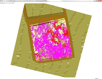
Figure 27a: Plot 1 visualized in smokeview at 1mX1mX1m (X,Y,Z) resolution with fire line portrayed in black. Note continuous fire line.
|
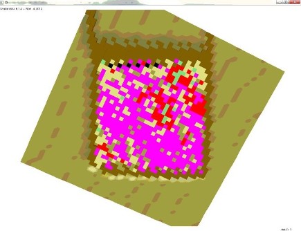
Figure 27b: Plot 1 visualized in smokeview at 4mX4mX1m (X,Y,Z) resolution with fire line portrayed in black. Note breaks in fire line.
|
GIS/Fire Model Integration Tutorials
The integration of GIS and Physics Based Fire Models is in it's infancy. As mentioned above, this is the first study that attempts to assess the feasibility of such an integration in a prescribed fire environment. The use of the WFDS-PB model requires competencies in the fields of fluid dynamics, thermodynamics, combustion and heat transfer. Testing the integration of geospatial data, such as that provided above, with WFDS-PB requires the above competencies along with competencies in geospatial science and technology, remote sensing, and LIDAR processing and analysis. Typically, the combined skills are not present in one individual requiring collaboration between Geospatial Professionals and Physics Based Fire Modelers.
The prototype software application facilitates integration of geospatial data with WFDS-PB. However, the appropriateness of this integration from a physics based modeling perspective might ultimately require modelers working with geospatial professionals to assess appropriate integration strategies such as those described above. Nonetheless, tutorials are presented below to demonstrate various integration possibilities using the current data.
The results of model simulations might provide valuable information on processing and transformation techniques required for GIS model integration.
However, the scale of analysis should be considered. For example, if the topographic knoll in plot 1 can be determined to be of a scale not relevant for analysis and building of the exposure scale (Maranghides and Mell 2012) or model validation, a flat terrain might suffice. Additionally, if the gentle sloping of topography from west to east can be determined to be of a scale not relevant for specific purposes, a flat terrain could suffice. The use of breaklines or smoothing operations as described above might also provide more appropriate inputs. Regardless, it is likely at this point that it will be an iterative process between Modelers and Geospatial Experts where various simulations are assessed and changes to geospatial inputs are made appropriately. Finally, without higher resolution analysis of the geospatial terrain products (i.e., use of DEMs with higher resolution in the Z direction) the question of appropriate processing and transformation techniques required for GIS and Fire Model Integration might remain unanswered. Other environments might be required for the analysis.
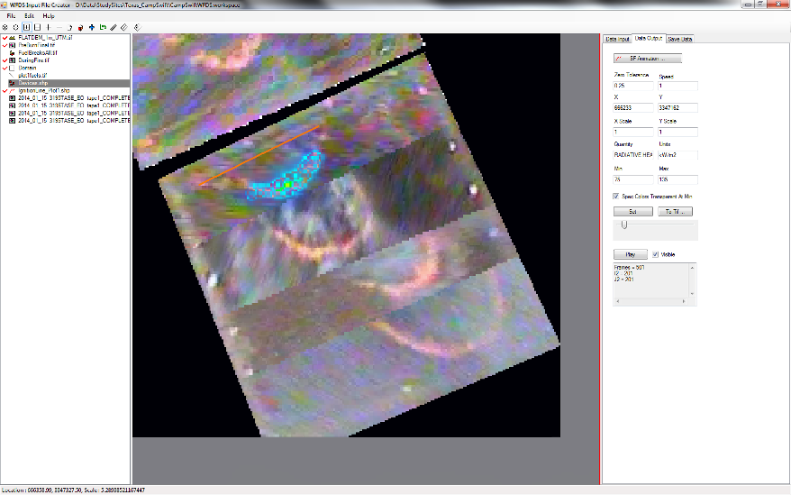
An example of fire model inputs and outputs viewed in an integrated environment available in the prototype software application is shown in Figure 28. Visualization tools like Smokeview provide valuable 3D animations. However, geospatial viewers such as those present in Figure 28 have potential to provide a more robust analysis environment allowing for further geospatial analysis and a more powerful viewing environment, and can be used in conjunction with Smokeview. Nonetheless, the prototype software application only demonstrates this potentiality and more enhancements are required for full exploitation of modeling and GIS technologies.
Some example WFDS input files created using the prototype software application can be downloaded below.
Summary and Recommendations
The data collected at research burns conducted at Camp Swift provides an excellent data set for the evaluation of science and technology related to characterizing fire at prescribed burns. This characterization provides a path forward for development of the Exposure Scale (Maranghides and Mell 2012). The use of geospatial technologies for the collection, organization and dissemination of data collected at prescribed burns provides an effective means for initial exploratory data analysis and data visualization. The use of a GIS to integrate the various spatial and tabular data collected during the Camp Swift burns for creation of WFDS input files is demonstrated above. Further study and model simulations are required to determine the appropriateness of geospatial data for WFDS inputs. It is expected this will be an iterative process between Modelers and Geospatial Professionals with many simulations required. The Camp Swift burns provide a plethora of data for this examination with only data for one of three plots being presented above.
Consequently, the above data, tutorials and WFDS input files are provided to modelers to help assess the feasibility of incorporating geospatial data into WFDS. From a geospatial perspective key items requiring additional study are as follows:
- Determining the relevant scale of interest for fire behavior and fire model validation.
- Identifying resolutions for geospatial data inputs required for fire model validation (i.e., grid cell resolution studies).
- Assessing grid cell resolution transformations for fuels that correctly allocate material properties of vegetation.
Additionally several recommendations for improving geospatial science and technology associated with prescribed burns are presented below.
GPS Improvements
Several improvements to the efficiency and effectiveness of GPS data collection are listed below:
- Collection of Fewer Higher Quality Points: the protocol used at the burns for GPS collection required collection of 180 points for each feature recorded. It can often times be more efficient to collect fewer points with higher quality position dilution of precision (PDOP) and other parameters. This might help achieve a horizontal accuracy closer to 10 centimeters while allowing for more efficient data collection.
- Use of an External Antenna: an external antenna might provide a clearer view of the sky and consequently a view to more satellites; thereby increasing the quality of points collected and possibly allowing for more efficient data collection.
- GLONASS Tracking: when utilizing base stations that use GPS and GLONASS data, enabling GLONASS tracking could both increase the accuracy of the data collected and increase the availability of H-Star accuracy. Using dual GPS/GLONASS receivers with antennas might also accelerate the time to first fix.
- H-Star Technology: the use of H-star technology would facilitate the collection of decimeter level accuracy data, if this is required.
- Record Images: associating images of features that are having locations recorded is a good practice and can help to reduce field data recording errors. Some of the ground control points were recorded well after the fire and ground control had been removed. In some cases this resulted in erroneous locations of ground control, which took a lot of time to discern, images of the features would have reduced the time it took to identify this field error. The field error was due to logistical difficulties associated with the burn.
It is important to understand that achieving accuracies stated in many GPS specifications require optimal conditions. For example, the limited concurrent GPS data available for Camp Swift does not indicate that 10cm accuracy was always achieved, although the accuracy was likely under 50cm and in many cases better than that, which is likely appropriate for the desired needs. This was likely due to less than optimal data collection conditions. Additionally, understanding specifications for vendor quoted accuracies in conjunction with project requirements is often important. Finally, it should be understood there will always be trade-offs between data quality and time of acquisition, which will require repeated use of the GPS unit to best understand.
Aerial and Ground Image Acquisition, and Ground Control Improvements
Several improvements to aerial image acquisition, ground image recording and ground control are as follows:
- Perform Camera Calibration: imagery from off-the shelf digital cameras might have distortion requiring the need for a camera calibration to determine the camera's interior orientation parameters. Calibration of visible and thermal video imagery might be conducted by placing grid patterns of ground control in a field and flying the UAV with the visible and thermal videos.
- Synchronize Camera Time and GPS Time: synchronization of the camera time with the GPS time will facilitate the creation of orthoimage products.
- Extend Ground Control Beyond Plots: extending the ground control beyond the plots and throughout the image acquisition area will aid in the quality of the ortho products produced.
- Use Smaller Ground Control for Still Images: fire shelters were established as ground control for visible video and were the only features available to use to georectify the DSLR imagery. Smaller ground control features (e.g. small boards with painted X's) could be utilized and more easily deployed across the study area of interest for DSLR imagery. Ensure the ground control is visible in the relevant sensor. These will also represent more spatially accurate ground control for high resolution DSLR imagery compared to fire shelters.
- Place Thermal Ground Control Further from Plot Edge: the thermal ground control became saturated as the fire approached these areas. Placing these further from the plot edge might reduce this effect.
- Place Ground Control within Plot: ground control within the plot will provide important data for validation. While thermal ground control within the plot might not be possible due to the possibility of it igniting the plot, visible video ground control could help validate locations of thermal video sensed heat release.
- Place Ground Control Evenly Around Plot: more ground control was placed on the east and west sides of the plots compared to the north and south. Taking some ground control from the east and west sides and moving to the north and south will present a better geometric arrangement of ground control for georectification or orthorectification.
- Determine Ground Sample Distance of Sensors: determine the ground sample distance of various sensors at various flying altitudes.
- Perform Quality Control of Imagery: a large advantage of a UAS over a fixed wing system is the ability to easily have multiple flights. Operators should perform established quality control procedures on collected images to quickly identify issues and re-fly as necessary. Before each burn commences operators should ensure equipment is functioning properly and fix, as possible.
- Output Video Stills: if ESD, MISB 0104.5, or MISB 0601 compliant metadata cannot be associated with video, it is recommended to output video stills at a higher frequency with associated times for enhanced data integration.
- Enhance Ground Image Collection: a greater amount of ground images are required for prescribed burns. All features should be photographed as described in the GPS section above. Additionally, newer technologies like PhotoSynth™ can be used to capture fuel plots and the area around sensors. In fact, the whole plot might be captured with PhotoSynth™ using a mobile device or similar technologies. Additionally, the use of more during fire ground images that image the same area from multiple angles would be very useful. The above could help create 3D point clouds of the plots that could be compared to UAS imagery derived point clouds and provide a better characterization of plot features. All imagery should be calibrated in regards to time. Recording of synchronized time with data is essential to model validation and fire behavior characterization.
- Associate GPS with Ground Images: all ground images taken should have a GPS position recorded. Cameras or devices with internal gps can facilitate this effort. However, this does not remove the need to sometimes explicitly associate an image or set of images with a particular feature recorded using a higher grade GPS unit.
The thermal infrared video was essential because of the ability to see through the smoke created by the fire. In some future burn plots, flying lower and utilizing the visible video and the thermal (to only record certain aspects of the fire) could help in understanding better the fire characteristics being sensed by the thermal sensor.
As discussed above certain above ground features will have distortions depending on the height and the camera angle. Creating what is termed a "true" orthoimage requires multiple images of the same location. In traditional photogrammetric mapping "true" orthoimages are produced to account for items such as building lean. Accounting for fire lean would also require multiple simulate nous views of the same area or more nadir viewing angles.
Data Management Improvements
The collection of data at prescribed burns is a multi-disciplinary effort requiring involvement from multiple organizations. This makes data management a difficult task. Nonetheless, several possible improvements to data management are listed below:
- Establish Consistent Nomenclature for Files: many files were named with dates using a different format. A consistent format should be used. It is recommended to use YYYYMMDD for file names that include a date.
- Establish Consistent Directory Structures for Data: the use of a consistent directory structure will aid in retrieval and archiving of data. Prescribed fire experiments could use the structure utilized by the National Wildfire Coordinating Group (GSTOP) or some other appropriate structure.
- Require Metadata from Data Providers: all data providers should have metadata describing the data. The project could decide on a consistent format for the metadata.
- Designate Specified Individual(s) for Data Integration: a individual or, depending on the size of the burns, a group of individuals should be in charge of data integration. These individuals should be present at the incident. GMS was not present at the incident. Being present at the incident would provide a better understanding of what occurred at the prescribed fires and result in more efficient and effective data integration.
Field Data Sampling and Remote Sensing Integration Improvements
Integration of field fuel sampling and remote sensing will facilitate a more thorough characterization of fire behavior and might result in better data inputs for model validation and fire behavior characterization. Some recommendations in this regard are suggested below:
- Collect Imagery Prior to Field Sampling: collection of imagery prior to field sampling will facilitate the possibility of extracting material properties of vegetation from imagery.
- Base Initial Sampling on Segmented Imagery: the pre-field sampling imagery can be segmented to allocate plot locations accordingly to ensure all fuel types are sampled. The image segmentation can then be improved based on field sampling.
- Perform Field Sampling within the Plots: pre-fire field sampling (not destructive) should occur within the plots. Simple transects can be conducted to help assess the accuracy of remote sensing classifications and provide a better understanding of plot fuels.
- Mark Sampling Plot Locations: ideally, marking the sampling plot locations with a well known point would aid in geolocation for accuracy assessments. This could present problems if the ground control effected the vegetation to be sampled. A flat item on a stake could solve the problem.
Finally, it is recommended that if the above fuel classifications are to be used for assessment that the sampled fuel plots that did not contain complete vegetation not be included in the assessment of material properties of vegetation for fire model inputs. The fuel classifications present above were very high resolution and consequently, fuel plots that contained only partial vegetation could misrepresent the material properties of vegetation if applied to a single fuel classification in the remote sensing derived fuels.
Future Work
Not only does the combined data provide a unique data set for fire behavior and fire model validation it presents a basic test to assess the integration of geospatial data and fire models. GMS will work with modelers to modify the above derivative products to assess appropriate processing and transformation techniques for GIS and fire model integration. Georectification of additional images while required is being conducted through a separate effort. This combined data can serve as an excellent initial case study from which more complicated integration strategies can be assessed (e.g. more complicated fuel and slope conditions).