GIS-WFDS Data Transfer

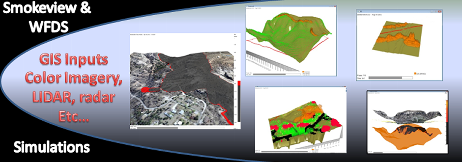
Transferring Geospatial Data to the Wildland Fire Dynamics Simulator (WFDS)

(National Institute of Standards and Technology Fire Research Grant 60NANB11D173)

Geospatial data can be described as data that has explicit geographic positioning information included within or associated with the data. Geospatial data can be divided into the following types of data:

1. Vector Data: vector data represents features using points, line or polygons. Vertices of features can record both the horizontal and vertical extent of the feature. Examples of fire model inputs that might be stored as vector data includes:

o Structure footprints stored as polygons portraying the boundary of the feature.
o Surface fuels stored as polygons portraying the boundary of surface vegetative fuels.
o Ignition locations stored as lines, points or polygons.
o Tree locations stored as points with associated attributes (e.g. height, crown width, etc…).
o Devices stored as points used to record model output information or otherwise display measurement devices.
o Model domains stored as polygons representing the boundaries of model simulations.

2. Raster Data: raster data can take different forms but is basically a matrix of 2D grid cells, often termed pixels, organized into rows and columns. Each grid cell has a value representing a particular phenomenon such as temperature or terrain elevation. Examples of fire model inputs that might be stored as raster data include:

o Terrain features represented as a continuous grid where each pixel has a numeric value representing the ground elevation.
o Boundary or surface fuels can also be stored as a raster data set where each pixel value represents a particular surface fuel type.
o Fuel elements or raised fuels can be represented as raster data where each pixel value contains the elevation of the top of the fuel. An associated raster data set representing the bottom of fuels or canopy base height can also be used to portray the vertical spatial extent of raised vegetation.
o Building heights can be portrayed in a raster data set where each pixel represents the height of the building at that location.

3. Tabular Data: both raster and vector data can have associated or sometimes related tabular data. Most vector data sets have a data table directly associated with the data set portraying information about the feature such as the tree height, crown width and other information. Raster data can also have an associated table portraying additional information about each pixel. Additionally, both raster and vector data can have data in related tables that stores information about that feature. For example, each ignition feature can have many records portraying features of the ignition at different times. A particular ignition line, for instance, might have a record indicating the ignition begins 10 seconds into the simulation. A separate record could indicate that at 15 seconds the heat release rate per unit area increases. Finally, at 20 seconds, the ignition line could have a record indicating the ignition ceases. Consequently, in the above case, the one record of a single ignition line can have three records portraying ignition characteristics. This is termed a one-to-many relationship.

An important transformation process for raster data representing terrain, building or vegetation heights to WFDS data structures involves taking 2.5D data, with a pixel value representing height, and transforming to 3D data structures or 3D grid cells with a dimension in the X, Y and Z directions. This transformation of terrain data from 2.5D grid cells to 3D grid cells will result in degradation of the input terrain and production of stair stepping artifacts as shown in Figure 1.

The degradation of the input data is a result of transferring to 3D grid cell structures. As shown in Figure 1, coarse grid cells will result in more abrupt and dramatic stair stepping than smaller grid cell sizes. Depending on the fire intensity, this could have repercussions for model simulations with higher intensity fires, in theory, being less susceptible to changes in simulation results at coarser grid cells compared to lower intensity fires.

Figure 2 Geospatial data transformations for surface fuels A). 7 centimeter horizontal resolution pre-fire imagery. B). Vegetation extracted from pre-fire imagery overlaid with 1 meter by 1 meter WFDS grid cells showing overestimation of no fuel areas when coarsening grid cell sizes. C). WFDS demonstration simulation showing the breaking up of the head fire coincident with areas of over exaggerated fuel breaks.

Figure 1 Cross-sectional diagram portraying transformation of 1 meter by 1 meter 2.5D digital elevation model (DEM) to 3D grid cells typical of data structures found in WFDS. A). Data transformation to 3 meter by 3 meter by 3 meter grid cells showing abrupt stair stepping. B). Data transformation to 1 meter by 1 meter by 1 meter grid cells showing generally less abrupt stair stepping but in some cases some smoothing should be performed.

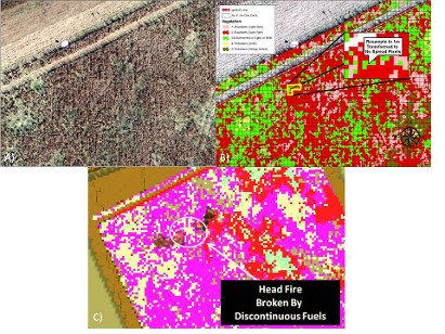
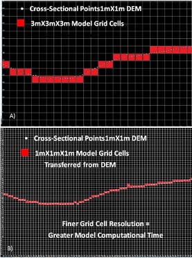
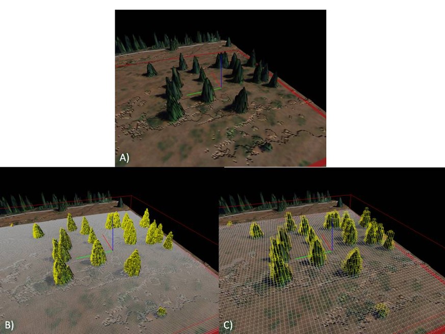
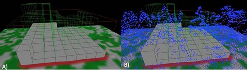
Transformation of surface fuel data to WFDS data structures can also result in data degradation. For instance, even a model run with 3D grid cell sizes of 1 meter by 1 meter by 1 meter over a domain of a few hundred meters by a few hundred meters can be computationally intensive. It is readily achievable, however, to acquire remote sensing imagery at 7 centimeters or less over significant areas as shown in Figure 2 above.

Classifying remote sensing imagery into fuel types can be achieved at high resolutions (e.g. 7 centimeters) as shown in Figure 2. Transferring surface fuel data to WFDS 3D grid cells using simple area weighted grid cell transformations can result in an over or under estimation of fuel load if the coarsened 3D grid cell encompasses several different surface fuel types in the original data. For example, as shown in Figure 2, coarsening the high resolution surface fuels to 1 meter by 1 meter by 1 meter 3D grid cells can result in 3D grid cells that contain both open/broomweed classification, having no or limited fuel properties that would be conducive to fire spread, along with blue stem classifications, where vegetative properties result in fire spreading readily through the vegetation.

When the respective coarsened grid cell takes the fuel type with the greatest area an underestimation or overestimation of fuel loads could occur. This data degradation might not be expected to simulate fire spread well compared to actual fire spread. Consequently, when the input fuel data set with seven centimeter horizontal resolution grid cells are transformed to coarser 3D grid cells some of the pixels that had fuels that would spread fire are all changed to no fuel spread in the coarsened grid cell.

This can artificially stop or break up fire spread as it no longer has the energy to cross these larger grid cells with no fuels as demonstrated in Figure 2c. A possible solution is to allocate the biomass based on area and not simply use the surface fuel type with the most pixels or area in a particular coarsened grid cell. Any solution will require data to assess the accuracy. Running at the full resolution of the fuel data is ultimately the best solution if computational demands can be met.

The applications developed for this project for transferring WFDS input data do not inherently handle the reallocation of biomass. The particular situation when to employ different grid resolution transformation techniques are not known given the lack of data currently publicly available. These transformations can, however, be handled in a GIS to create new input data sets from which WFDS input files can be created using the WFDS Input File Creator software. Ultimately, making research data collected for prescribed burns publically available will be required to better understand specific transformation requirements and incorporate these into the WFDS Input File Creator.

Transforming geospatial data inputs representing raised fuel elements or above ground vegetation from active sensors such as LIDAR to coarser resolution 3D grid cells will also degrade the data. This data degradation can be seen in Figure 3a portraying a LIDAR derived canopy height model (CHM) in 3D overlaid on a relatively flat terrain for a project study site at Joint Base Lewis McChord. Figure 3b shows that the CHM transformed to 3D grid cells at 1 meter resolution will have a tighter fit to the input LIDAR derived CHM compared to 3D grid cells at 3 meter resolution.

Figure 3 LIDAR CHM transferred to 3D WFDS grid cells at different resolutions using WFDS Input File Creator. A). LIDAR derived CHM extruded (green coned shaped structures) above ground surface overlaid on aerial image. B). LIDAR terrain and vegetation overlaid with WFDS grid cells for vegetation (yellow) and terrain (white) at 1 meter by 1 meter by 1 meter grid cell sizes. C). LIDAR terrain and vegetation overlaid with WFDS grid cells for vegetation and terrain at 3 meter by 3 meter by 3 meter grid cell sizes.

This data degradation at 3 meter resolution can be seen when comparing Figure 3b with Figure 3c. The extruded CHM (green) when overlaid with 3D grid cells of 3 meter resolution can be seen through the overlay but at 1 meter resolution the CHM grid cells more closely fit the underlying CHM as evidenced by more space being visible through the overlay as opposed to the CHM filling the overlay. In this case, if not accounted for, the data degradation when coarsening grid cell sizes would result in overestimation of biomass.

The degradation of data shown in Figure 3 is more difficult to overcome compared to degradation from 2D transformations for boundary fuels. The consequences could be significant as described in Parsons et al (2011)[i]. Depending on the consequences for fire behavior, the spatial heterogeneity of the tree canopy might still not be captured at 1 meter 3D grid cell resolutions. Approaches such as described in Parsons et al (2016)[ii] for the STANDFIRE fuel and fire modeling system could be required to model canopy distributions but remain unfounded. STANDFIRE also does not provide tools for integration of geospatial data such as the tools developed for this project including terrain. Nor does STANDFIRE provide mechanisms to transfer modeled vegetative stands to real-world landscapes.

Nonetheless, a solution to calculate the volume occupied by original grid cells in comparison to new grid cells could be required for integration with both functional aspects of STANDFIRE and the WFDS Input File Creator. This might allow for appropriate recalculation of biomass for vegetation and allocation of properties to coarsened grid cells based on volume occupied by the original data. Regardless of the method, it appears that modelers should be careful when changing grid cell sizes. Some coarsening can result in very inappropriate representations of spatial features.

Figure 4 TIN of a CHM for a portion of a WUI community displayed in prototype WFDS Input File Creator.

One technique that was explored in this study involved the use of a Triangulated Irregular Network (TIN) as shown in Figure 4. TIN functionality was incorporated into the prototype WFDS Input File Creator to examine the possible solution of calculating volumes betweens TINs (Canopy Height Model and Bare Earth DEM) produced at different resolutions. The situation, however, is more complicated for WFDS as the area of the TIN occupied by each grid cell needs to be calculated as shown in Figure 5. This is a computationally expensive calculation, the specific algorithms of which have not been determined. Furthermore, limited field data exists for the validation of such a method and the functionality was not incorporated into the final WFDS Input File Creator.

Figure 5 A single WFDS grid cell at 5 meter resolution. Green shapes indicate the TIN of the CHM model for this particular grid cell as displayed in the prototype WFDS Input File Creator and black areas represent grid cell areas not occupied by vegetation.

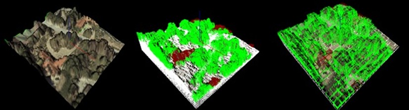
Additionally, as grid cell sizes are coarsened a single grid cell might contain more than one feature from the original resolution data. This is shown in Figure 13 portraying LIDAR derived vegetation, buildings and terrain for a small area in a WUI community in Southern California (The Trails at Rancho Bernardo). As can be seen in the images in Figure 13, finer resolution 3D grid cells (e.g. 1 meter) will result in a tighter fit to the underlying height data and less mixed feature grid cells compared to coarse resolution 3D grid cells.

Also, coarser grid cell resolutions (e.g. 5 meters) can result in features being lost as is shown in Figure 6 where the building 3D grid cells (red) are encompassed by the vegetation grid cells (green). It is an arbitrary choice which feature will be lost, except for the fact that WFDS will override any fuel element grid cells with obstacles (terrain or sometimes buildings) when there is overlap. In some cases the data might need to be developed in a GIS in a different manner depending on the environment and intended purpose of the simulation.

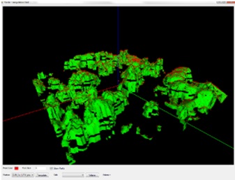
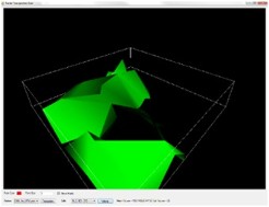
Figure 6 3D images of the Trails LIDAR data overlaid with aerial images. The first image shows the LIDAR data in a 3D environment with an aerial image overlaid. The second image shows the same data with 1 meter resolution 3D grid cells overlaid. The third image shows the raw LIDAR data in combination with 3D grid cells at 5 meter resolution. There is more empty space between grid cells and underlying height models at 5 meter resolution compared to 1 meter resolution and building features (red-brown) are encompassed by vegetation (green) grid cells at the 5 meter resolution case.

The stair stepping artifacts produced as a result of transforming 2.5D terrain data to 3D data structures also has consequences for accounting for vegetation height. For example, the stair stepping that is produced when performing terrain data transformations can result in abrupt height jumps in terrain over otherwise relatively flat slopes. This is shown in Figure 6 below with 3 meter resolution grid cells of terrain shown in grey. At some point the gradual increase or decrease in height on a relatively flat slope will produce a height jump as shown in Figure 6.

Figure 6 3D grid cells at 3 meter resolution overlaid on terrain (green = vegetation, grey = terrain, blue = LIDAR vegetation returns). A). Portrays abrupt and artificial jump in elevation due to the coarse grid cell size (3 meters) over a gently sloping terrain. B). Portrays 3D grid cells at 3 meter resolution with LIDAR returns from vegetation showing some 3D grid cells at top of canopy having no returns from the LIDAR. Download animation of above figure.

If this height jump location contains above ground vegetation the transformation to 3D grid cells must make a decision to retain biomass of the vegetation and artificially raise the height of vegetation along the height jump or have no vegetation height jump and reduce vegetation biomass. Current implementations of the final WFDS Input File Creator produce an abrupt jump in vegetation height and maintain the input biomass of the vegetation as shown in Figure 6[1]. As shown in Figure 6, portraying LIDAR point returns along with 3 meter resolution 3D grid cells, the height jump can result in grid cells with no actual data portraying vegetation.

The above highlights the difficulty of using coarse grid cells in certain environments. Relatively gently sloping terrain can use dynamic surfaces and breaklines to reduce abrupt stair stepping in certain locations. The fire line depth of WFDS simulations needs to be covered by 3 grid cells as a rule of thumb. Consequently, the resolution of the fire line that will drive the resolution requirements of other data inputs to WFDS, among other factors.

[1] Building the data up differently in a GIS could help alleviate this, which is one reason for the loose coupling employed between WFDS and the geospatial viewer developed for this project that takes advantage of the power of GIS while providing a simpler tool for data transfer.

[i] Parsons RA, Mell WE; McCauley P (2011) Linking 3d Spatial Models Of Fuels And Fire: Effects Of Spatial Heterogeneity On Fire Behavior. Ecological Modeling 222:679-691.
[ii] Parsons RA, Wells L, Pimont F, Jolly M, Linn R, Mell W (2016) “STANDFIRE: An IFT-DSS Module for Spatially Explicit, 3D Fuel Treatment Analysis.” Final Report for JFSP Project 12-1-03-30.